= ЭЛЕМЕНТАРНЫЕ ЧАСТИЦЫ И ПОЛЯ
FINAL STATE INTERACTION EFFECTS
IN B0 ^ J/фж0 DECAY
© 2014 Hossein Mehraban*, Amin Asadi**
Physics Department, Semnan University, Iran Received May 5, 2014
In this research the exclusive decay of B0 ^ J/^п0 is calculated by QCD factorization (QCDF) method and final-state interaction (FSI). First, the B0 ^ J/^п0 decay is calculated via QCDF method. The result that is found by using the QCDF method is less than the experimental result. So FSI is considered to solve the B0 ^ J/^п0 decay. For this decay, the D+D-* and D0D0* via the exchange of D-, D-* and D0, D0* mesons are chosen for the intermediate states. The above intermediate states are calculated by using the QCDF method. The experimental branching ratio of B0 ^ J/^п0 decay is (1.76 ± 0.16) x 10-5 and our results calculated by QCDF and FSI are (0.56 ± 0.11) x 10-5 and (1.3 ± 0.09) x 10-5, respectively.
DOI: 10.7868/S0044002714120137
1. INTRODUCTION
The importance of final-state interaction (FSI) in weak non-leptonic B-meson decays is investigated by using a relativistic chiral unitary approach based on coupled channels [1—3]. The chiral Lagrangian approach is proved to be reliable for evaluating hadronic processes, but there are too many free parameters which are determined by fitting data, so that its applications are much constrained. Therefore we have tried to look for some simplified models which can give rise to reasonable estimation of FSI [4, 5]. The FSI can be considered as a re-scattering process of some intermediate two-body states with one-particle exchange in the t channel and computed via the absorptive part of the hadronic-loop-level (HLL) diagrams. The calculation with the singlemeson-exchange scenario is obviously much simpler and straightforward. Moreover, some theoretical uncertainties are included in an off-shell form factor which modifies the effective vertices. Since the particle exchanged in the t channel is off shell and since final-state particles are hard, form factors or cut-offs must be introduced to the strong vertices to render the calculation meaningful in perturbation theory. If the intermediate two-body mesons are hard enough, so that the perturbative calculation can make sense and works perfectly well, but the FSI can be modelled as the soft re-scattering of the intermediate mesons. When one or two intermediate mesons can reach a low-energy region where they
E-mail: hmehraban@semnan.ac.ir
E-mail: amin_asadi66@yahoo.com
are not sufficiently hard, one can be convinced that at this region the perturbative QCD approach fails or cannot result in reasonable values. If the intermediate mesons are soft, one can conjecture that at this region the non-perturbative QCD would dominate, and it could be attributed into the FSI effects. Because all FSI processes are concerning non-perturbative QCD [6], we have to rely on phenomenological models to analyze the FSI effects in certain reactions. In fact, after weak decays of heavy mesons, the particles produced can re-scatter into other particle states through non-perturbative strong interaction. We calculated the B0 — decay according to
the QCD factorization (QCDF) method and selected the leading-order Wilson coefficients at the scale mb and obtained the BR (B0 — J/^n0) = (0.56 ± ± 0.11) x 10-5. The FSI can give sizable corrections, and we utilize it [7]. Re-scattering amplitude can be derived by calculating the absorptive part of triangle diagrams. In this case, intermediate states are D+, D-* and D0, D0*. Then, we calculated the B0 —
— decay according to the HLL method. Taken FSI corrections into account, the branching ratio of B0 — J/^n0 becomes (1.3 ± 0.09) x 10-5 and the experimental result of this decay is (1.76 ± 0.16) x x 10-5 [8].
This paper is organized as follows. We present the calculation of QCDF for B0 — decay in
Section 2. In Section 3 we calculate the amplitudes of the intermediate states of B0 — D+D-* and B0 —
— D0D0* decays. Then we present the calculation of HLL for B0 — decay in Section 4. In Section
1555
4*
J/W
•wxr
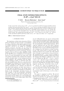
Fig. 1. The Feynman diagrams for B0 ^ J/^n0 decay.
5 we give the numerical results, and in the last section we have a short conclusion.
2. QCD FACTORIZATION OF B0 — DECAY
In the generalized factorization approach, the B0 — J/^n0 decay has color-suppressed tree and allowed penguin diagrams to B0 — decay.
The diagrams describing this decay are shown in Fig. 1.
According to the QCDF the amplitude of B0 — — decay is given by
Aqcd(B° ^ j/^n0) =
—iV^Gpnij/^(ej/tf, ■PB)fwA^J/'1' x
(1)
X [VcbVcdaz + Xp[aa + rJ^(a5 + a7 + a9)]},
where Xp are the products of elements of the quark-mixing matrix. Using the unitarity relation \p + Ac + + Xt = 0, we write
(2)
\ = VpbVpd,
p=u,c
and for vector meson J/^ the ratio r'J/^ is defined as
=
' x
mb fj/^
(3)
3.1. B0 — D+D-* andB0 — D0D0* Decays
When two intermediate mesons exchange d quark and two final-state mesons exchange s quark, the D+ and D-* mesons are produced for intermediate state via exchange mesons of D- and D-*. If u quark is exchanged between two intermediate mesons and s quark is exchanged between two final-state mesons, the D0 and D0* mesons are produced for an intermediate state via D0 and D0* as the exchange mesons.
For B0 — D+D-* decays, Feynman diagrams are shown in Fig. 2, and the amplitudes read
A(B0 — D+D-*) = (4)
= -iV2GFfDmD*{sD* ■pB) x
x ABBd* {(ai + a2)VcbbV:d + Gp
+ [a,4 + aio + (a6 + a8)Xp}} + i—=fBfDfD* x
V2J
M biVcb +
b-i + 264 — -b-ieW + -bieW
where
(5)
3. AMPLITUDES OF INTERMEDIATE STATES
In this section, before analyzing FSI in the B0 ^ ^ decay, we introduce the factorization ap-
proach in detail. The effective weak Hamiltonian for B decays consists of a sum of local operators Qi multiplied by QCDF coefficients Ci and products of elements of the quark-mixing matrix [9]. The factorization approach of the heavy-meson decays can be expressed in terms of different topologies of various decay mechanisms such as tree, penguin, and annihilation.
61 =
C3AI + C5 (A3 + A3) + NcC6Al C9 Ai + cz(A3 + A3) + NcC8A3
h,eW = [cwA\ + CgAl] ,
where Ci are the Wilson coefficients, Nc is the color number and
Cf
*> = h Cf
W = jç
9(A^-4 + ^)+rfrf Xi
A3 = 0,
A3 = 2nas (rD+ + rD°*) (2X\ - XA) ,
, (6)
c
b
d
\
p
D+
d
D+
D-
D-
d _ W b
D-
D-
D+
W-
(D+)D-
(D+)D-
D-'(D+)
Fig. 2. The Feynman diagrams for B0
D-
al = ef + —c%1 (i = odd),
eff
N
(7)
D (D+) d
^ d+ d-* decay.
x M(B — MiM2)G(MiM2 — M3M4),
Oi = 4 + — d_ 1 (i = even),
where f runs from f = 1, ..., 10 and ai and a2 are both related to the coefficients c1 and c2, which are very large compared to other Wilson coefficients. The process of the B0 — D°D°* decay only occurs via annihilation between b and d; for these decays Feynman diagrams are shown in Fig. 3, and the amplitudes read
A(B0 — D°D°*) = (8)
Gp
= i — ÎBfDÎD*{bi + 264 + 2&4eW/')Ap.
for which both intermediate mesons (Mi, M2) are pseudoscalar. And the absorptive part of the HLL diagrams for VP case can be calculated as
Abs M (B (pb ) — M (pi)M (p2) — (10) — M (ps)M (P4)) = _ 1 f d3 pi d3p2 ~ 2 J 2Ei(2ir)3 2E2{2ir)3 X
x (2n)45a(pb - Pi - P2)Vckm x x {2am(e*v ■ pb)(fpA$^V + fvFB^p) + + fB fp fv bi}G(Mi M2 — M3 M4),
4. FINAL STATE INTERACTION OF B0 — J/^n0 DECAY
For B0 — decay, two-body intermediate defined as
state such as D+D-* and D0D0* is produced. We can write out the decay amplitude involving HLL contributions with the following formula
where M(B — M1M2) is the amplitude of B — — M1M2 decay calculated via QCDF method and G(M1 M2 — M3M4) involves hadronic vertices factor
(11)
Abs M (B (pb ) - M (pi)M (p2 ) - (9)
- M(p3)M(p4)) =
1 f d3pi d3 p2 . .44, ,
2 J 2Ei(2ir)3 2E2(2ir)3 ЫРв-Рг-ъ)*
{В(рз)ф(£2 ,P2)\iF\D(pi)) = = -ig^DDе2 • (Pi + Рз), (D*(s3,p3}iP(s2,p2)\id\D(Pl)) =
{Б*(ез,рзЖе2 ,P2)\iF\D*(ei ,pi)) = -ießе2el [2pivgaß - (pi + P2)agvß + 2p2ßgav].
+
D
b
0
в
0
в
d
b
c
d
d
t
g
0
0
в
D
в
0
в
+
D
+
0
0
в
0
в
в
c(u )
D (D )
D0(D0 )
D0 (D0)
D0*(D0)
Fig. 3. The Feynman diagrams for B° d°d°* decay.
D+
d d
Fig. 4. Quark level diagram for B° ^ d+ d * ^ j/^n° decay.
The dispersive part of the rescattering amplitude can be obtained from the absorptive part via the dispersion relation [6, 10]:
Dis M(m'ß) = - f^-n J s'
AbsM^S', (12)
s — m
in B° D+D-
J/^n Decay
the mode
B0 ^ D+(Vl)D-*(e2,V2) ^ ,ps)n°(VA)
is given by
B
where s' is the square of the momentum carried by the exchanged particle and s is the threshold of intermediate states, in this case s ~ m2B. Unlike the absorptive part, the dispersive contribution suffers from the large uncertainties arising from the complicated integration.
4.1. Final State Interaction
The quark model diagram for B0 — D+D-* — — decay is shown in Fig. 4. The hadronic-
level diagrams are shown in Fig. 5. The amplitude of
Abs(4a) =
d3pi d3p2
-iG F
2y/2 J 2E1(2tt)s 2E2(2TT)s i
x (13)
X (2n)4Ö4(vb - Vi - V2)(-ig^DD)£3 • (vi + q) x X (-igDD*n)£2 • (-q)\ 2mD* (£2 • Vi)IdAbd* x
x [(ai + a2)VcbV*d + (a4 + rx (a6 + as) + aio)Ap] -
- fB fD fD*
biVcbVc*d + ( 63 + 264 - -hew +
+ £ bieW ) Ap
\F'\q\m2D) iGp
J Ti Ssf2nmB X
0
B
b
0
D
B
d
d
s
—
a b
J/W
D-
J/W
Fig. 5. The hadronic level diagrams for B0 ^ d+d * ^ j/^n0 decay.
X g^DD gDD* * J |Pi|d(cos 0)^2H2mD* fD ABD* x -i
x [(ai + a2)VcbVcd + (a4 + r£(a6 + as) + aw)\p] -
- fB fD fD*
blVcbV*d + (63 + 264 - 2b3eW +
1,
Hi
F2{q2,m2D) Ti
Here,
Hi = (£3 ■ Pi)£ ■ P4)= (14)
f EM - E3\Pl\ cos d\f E4\p2\ - E2\p4\ cos 9
V rnB\p3\ A mB\P2\
H2 = (£2 ■ Pi)(£2 ■ P4)(£3 ■ Pi) =
. (Pi ■ P2)(P2 ■ P4)\
Pi ■ p4 H--5- 1 x
m2Dt
x iEM-E-McosO V rnB\p3\
Ti = (pi - P3)2 - mD = = pP{ + p3 - 2p°p° + 2pi ■ p3 - mD, q2 = m2 + m23 - 2EiE3 + 2|Pi||P3| cos 6 = = mD + mJ^ - 2p°ip0 + 2pi||p3| cos 6,
6 is the angel between pi and p3, q is the momentum of the exchanged D- meson, and F(q2,m2D) is the form factor defined to take care of the off-shell exchanged
Для дальнейшего прочтения статьи необходимо приобрести полный текст. Статьи высылаются в формате PDF на указанную при оплате почту. Время доставки составляет менее 10 минут. Стоимость одной статьи — 150 рублей.