APHydro2014
cyflOCTPOEHMi 6'2014
Measurement of Sloshing Flow Using Particle Image Velocimetry
Jieung Kim*, Jae-Han Kim**, Sang-Yeob Kim* and Yonghwan Kim*' ^Department of Naval Architecture and Ocean Engineering, Seoul National Univ ersity
Seoul, Korea
**Daewoo Shipbuilding & Marine Engineering Co. Ltd Seoul, Korea tyhwankim@snu.ac.kr
ABSTRACT
In this study, a particle image velocimetry(PIV) technique is used for measuring the velocity vectors of sloshing flow, and the measured velocity fields are compared with those of an analytic solution. For this PTV experiment, a two-dimensional rectangular tank and two high speed cameras are installed on motion platform. Various image capturing methods and filtering sehemes are used for velocity vector analysis. The velocity vectors of fluid flow are compared between experimental data and analytic solutions.
KEY WORDS: PIV, Sloshing, Standing wave, flow measurement
INTRODUCTION
As sloshing analysis is an essential element in LNG ship cargo design, fluid flows in partially filled tank have been studied actively based on experimental, semi-analytic and numerical methods. Because of the
experimental, semi-analytic and numerical methods. Because of the strong non-linearity of physical phenomena, sloshing problems were preferably studied by experimental way rather than numerical method. Particularly, sloshing-induced impact pressure has been the main interest for the structural assessment of LNG CCS(cargo containment system). Recently, velocity measurement in sloshing flow is of interest, since people are getting interested in the correlation between velocity and dynamic pressure. H'or instant, Gavory (2005) suggested to use a PIV technique for the velocity measurement of violent sloshing flow. There are a few existing studies adopted PIV technique in sloshing experiment. Lugni el al. (2006) measured pressure and velocity in flip through of sloshing using PIV. Doh et al. (2011) used PTV for evaluating the occurrence of sloshing. Ahn et al. (2012) measured oscillating characteristics of pressure and velocity using PIV in Ihe case of trapped air at the tank roof. Likewise there have been various research on PIV applied on sloshing, but it is hard to find three-dimensional PTV measurements for sloshing flow. Recently, PIV system has been equipped in SNU sloshing tank for measuring three-dimensional sloshing flows.
cyWOCÏPOEHVIE 6'2014
APHydro2014
This paper introduces the first study which was focuscd on two-dimensional measurement. In this study, a newly established PTV system has been validated for standing wave case which has weak non-linearity. The model tank used in this experiment is a transparent acrylic tank which can make it available to observe internal fluid flow, but the tank beam is narrow so that sloshing flow is nearly two-dimensional. Excitation condition has been chosen as tie steady standing wave could be generated.
Using captured images, the comparison of experimental results and linear analytic solution has been made in different excitation conditions. Flow images are captured in 100FPS(frame per second) in each camera and extraction rate is choscn as 10. 20. 50 and 100 FPSs. Additionallv. filtering effect on the experimental result was observed in the analysis of velocity vectors.
THEORETICAL BACKGROUNDS Principle of Particle linage Velocimetry
P1V is an experimental method which measures fluid velocity field by capturing the images of illuminating particles. In PIV system, the displacements of particles within interrogation area are computed using cross-correlation between two adjacent images as follows:
c(s) = (A'+
(1)
where, C(.S) is cross-correlation function, Ar is interrogation area and J is intensity function of position X . Specific S which makes C(.S) maximum is regarded as displacement. Consequently, velocity vector can be calculated by dividing the displacement by time interval between two images (Prasad, 2000).
Filtering Scheme
When correlation between two images is computed, there may be some errors due to the uncertainty of particle intensity or other reasons. To correct the error vectors, a filtering algorithm can be used to mitigate the effects of such error sources. In this study, an average filtering schcmc and a cohcrcncc filtering scheme arc applied in post processing. The average filter calculates the average of surrounding vcctors in a specified area, and it is considered as flow vector(see Fig. 1(a)). In the case of the coherence filter, a velocity vector is revised if it is erratic compared with surrounding flow tendency.
0 0 0 0 ... 0... Q
Vector being filtered
(a) Average filter (b) Cohcrcncc filter
Fig. I. Ranges of two different filtering processes
To apply the cohcrcncc filter, all Ihc vcclors within a specified area of filtering radius R, as shown in Fig.1(b), are considered to compute the mean cumulative difference A, of certain vector v,- which can be defined as:
z IF --
A, =-
n-\
(2)
Then the vector with minimum mean cumulative difference value, vmcj , becomes median vector which characterizes the representative velocity.
If difference between vc and v„„i is larger than minimum mean cumulative difference, then v, is substituted by the median vector. Otherwise, vc is remained as original value. This series of process can be expressed as follows (Chetverikov, 2003):
(3)
if ||v, -iw||>Amai
I v<-aw = v<- if |vc. - Vw I < A^
Comparison between PIV Data and Analytic Solution
In this study, the experimental results of standing wave are compared to linear analytic solutions (Kim, 2003). Let's consider a partially-filled 2D rectangular tank and a coordinate system, as shown in Fig. 2:
Harmonic motion <->
Model lank
\
Field of view
Fig, 2, Coordinate system for experiment and analytic solution
When the model tank is cxcitcd to have onc-dimcnsional harmonic translational motion, the velocity potential in fluid domain can be written as:
V . ., , lY] Je~T' A cos(wt) + Bsin( " /)!
^=2Jsm *■»' i I l™511^)1 J|
n—Q 1 [ C„ cos(oi) + D sm(ii)/)
= —c — K„
4
k_ = —
L [ (2n - 1)ti
1- (-T
(t)A
cosh {(2n - l)7th/Lj
K^lijBJto;
a„l.2
tod„
(a)2 -®*)2 + |i,(o* (V - in2 J + f,i ¡i
(4)
where, L. h, w, g are the length of model tank, water depth, oscillation frequency, and gravity acceleration, respectively, fti is an equivalent linear damping coefficient, and it is set up to 10% of critical damping in this study. By differentiating the velocity potential, velocity vectors in fluid domain can be obtained. To compare experimental results and analytic solution quantitatively, DF is defined as follows:
DF = Z
D.,
' n '
D, --
I'M
(5)
where D: refers to the normalized difference of velocity vector, Vis velocity calculated from the analytic solution, [■',, is the velocity obtained from the experiment, F„,„ is the maximum velocity of the analytic solution, and n is the number of velocity vectors to be observed. DF can be calculated in two different aspects; position-fixed and time-fixed analyses, In the position-fixed concept, DF indicates the average of each velocity difference, which varies with respect to time at a ccrtain location. The calculating range is one time period and
APHydho2014
СУДОСТРОЕНИЕ 6'2014
CVÄOCTPOEHWE 6'2014
APHydro2014
APHydro2014
cyflOCTPOEHMi 6'2014
Time Fixed Analysis
Figs. 16 and 17 indicate DF values with respeet to capturing speed for two time instants. It can be seen that DF value in tpos is higher than in tneg due to peak diffcrcncc in experimental result. Moreover, the graphs show that filtering does not change the DF values significantly, because DF is an averaged parameter and filtering analysis changes only few error vectors.
Still, it can be confirmed that both of average filter and coherence filter affect velocity vector map. For instance, in the case of 50FPS Bosens camera tnel. velocity vcctor map obtained by correlation is presented in Fig. 1 8, It can be seen that some vectors do not follow the overall flow tendency.
0,8
v.! U.O U. S □ U.4 U.J
u.i
V.I
0
Coherence Average
0
-tl-
JQ . 40-60 SO-LOO.
©
20-4Ü-60-KÜ-
i_aplu. .rig seocd(i 'S)
(a) Y4 camera (b) Eos ens camera
Fig. 16. DF with respect to FPS for time fixed analysis at t^
0-8
0.7
0-6
0.5
LL. D 0,4
0.3
0.3
0.1
0
Raw n Coherence Average
-
J_
3 & |
1— ft— ■fi— 1«- A—t HH-
0,7 Rav □ CW A Avi
0.6
9.5 J
0.4
0.3
0,2
O.lf 1 e 3
0 —» G h—41 fr~H n-1
(.(iplunng speedy i*S) (a) Y4 camera
Capturing speedl.rrS) (b) Eosens camera
Fig. 17. DF with respect to FPS for position fixed analysis at tn6
TTTTTJ
i ill Mi fl iI11
(a) Vectors overlapped on image
[i. x(nun)
(b) Numerically exported vectors
Fig. 18. Velocity vector map obtained by correlation based calculation
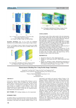
When two filters arc applied to this raw velocity vcctor map, vector map changes into as shown in Fig. 19(a) and Fig. 19(b). In these figures, sohd vectors are raw data and dashed vectors are filtered vectors. Bo1h figures show that error vectors are replaced into appropriate velocity vectors, but the vector maps are slightly different. In the average filter, error vectors affect surrounding vcctoTs because the error vector's arc also included in averaging other vectors, hi the coherence filter, however, error vectors have an insignificant effect on surrounding vectors. Thus, the coherence filter is preferred than the average filter in post processing.
-27 -28
S -29 5
TTTTTJ
! ill I I I N I I I / / ' I ill I
-22 x(mm) (a) average filter
E -29
J,
-30
TTTTTT
I ill 11 N i I I I I I I
-24
-22 x(mm) (b) coherence filter
Fig. 19. Comparison of velocity vector map between raw data and liltercd data
CONCLUSIONS
In this study, a two-dimensional tank experiment which generates standing wave has been performed, and velocity vectors are measured by using a P1V system. Based on this st
Для дальнейшего прочтения статьи необходимо приобрести полный текст. Статьи высылаются в формате PDF на указанную при оплате почту. Время доставки составляет менее 10 минут. Стоимость одной статьи — 150 рублей.