ЯДЕРНАЯ ФИЗИКА, 2014, том 77, № 3, с. 399-408
ЯДРА
NEW METHOD FOR SOLUTION OF COUPLED RADIAL SCHRODINGER EQUATIONS: APPLICATION TO THE BORROMEAN TWO-NEUTRON HALO NUCLEUS 22C
© 2014 S. N. Ershov1)*, J. S. Vaagen2), M. V. Zhukov3)
Received January 29, 2013
A generalized PrUfer transformation within the framework of the modified variable phase method has been used for numerical solution of coupled radial Schrodinger equations at negative energies. The method has been applied to calculations of the Borromean two-neutron halo nucleus 22 C, for which an unusually large value of the matter radius has recently been extracted from measured reaction cross sections. The giant size can only be explained by an extremely loose binding that is, however, not yet known experimentally. Within the three-body cluster model we have explored the sensitivity of the 22 C matter and charge radii and soft dipole mode excitations to the two-neutron separation energy.
DOI: 10.7868/S0044002714030076
We cordially dedicate this work to Vladimir B. Belyaev on the occasion of his 80th birthday
1. INTRODUCTION
The Schro dinger equation of quantum mechanical systems is often converted into a system of coupled radial equations, with applications in nuclear physics, quantum chemistry, etc. A variety of solution methods for such systems has been developed. Recently, new methods for solution of coupled equations were suggested [1, 2]. These methods contain rearrangement of the original set of equations into a new set which is more appropriate for maintaining the linear independence of the solution vectors. The realization of the idea of the rearrangement was different in the two papers [1, 2]. In the first [1], the full radial interval is split into finite intervals, and then the radial equations are rearranged on each interval to avoid numerical instabilities. Finally, the global solutions are constructed from the local solutions. In the second article [2] the same idea of coupled equations rearrangement is applied to the variable phase method for solutions of Schrodinger equations. This second realization is simpler and numerically more effective than the first one. Still, when the modified variable
1)1 Joint Institute for Nuclear Research, Dubna, Russia.
2)Institute of Physics and Technology, University of Bergen, Norway.
3) Fundamental Physics, Chalmers University of Technology, Goteborg, Sweden.
E-mail: ershov@theor.jinr.ru
phase method is applied for finding the bound state solutions in cases of deep potentials, some numerical difficulties may appear. To remedy this drawback a new modification, that uses a generalized Priifer transformation [3—5], is suggested.
The new method is applied for exploration of the 22 C nuclear structure. Recently, the matter radius of this heaviest known Borromean two-neutron halo nucleus was extracted [6] from measured reaction cross sections: a giant matter radius of 5.4 ± 0.9 fm. Theoretical implications of this finding, if correct, need however to be investigated. The nuclear size is intimately connected to the energy of the lowest breakup threshold. The value of the two-neutron separation energy is not experimentally known and the last evaluation [7] assigns for 22C a rather uncertain value, S2n = 0.42 ± 0.94 MeV. Such an ambiguity has fueled discussions [8, 9] about 22C possibly having extremely large size. Below we discuss our new solution method and the influence of the binding energy on the matter and Coulomb radii, and on the soft dipole excitations, using 22 C as example. The nuclear structure of 22C is considered in the framework of a (20C + n + n) three-body model applying the hyperspherical harmonic (HH) method [10, 11].
2. SOLUTION OF THE COUPLED RADIAL SCHRO DINGER EQUATIONS
The system of N coupled radial Schro dinger equations may be written as
f d2 2mE U{U + l)\
{-^ + —2---—)M= (1)
N
j=1
where E is a total energy and Li is the orbital angular momentum in channel i. The first index of ^in(r) denotes the ith component of a wave function (i = = 1,..., N), while the second index n marks different linear independent solutions. The N x N matrix of coupling potentials Vij(r) is assumed symmetric, i.e. Vij(r) = V,(r). Note that the potentials include the factor 2m/h2 and have the dimension fm-2. Only solutions that satisfy definite boundary conditions imposed at the origin and at infinity have physical meaning. For bound states (E < 0) the boundary conditions demand that wave functions have regular behavior at the origin and decay exponentially for large values of r
^in(r ^ 0) ^ 0, ^in(r ^to) ^ exp(-kr), (2)
where k = ^/2m\E\/h2.
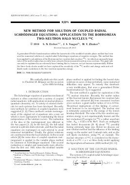
The general method to solve the boundary value problem for coupled equations (1) consists of two steps. First, sets of linear independent solutions are calculated and then, exploiting the linearity of the coupled equations, a suitable combination of different sets with the required boundary conditions, is found. To perform the first task the coupled equations have to be integrated with linear independent initial values to get the linear independent solutions. A major problem in numerical solution is the difficulty of maintaining the linear independence of the solution vectors in the process of numerical integration. Troubles come from the existence of radial regions where some components of the wave function are classically forbidden and others are not. Figure 1 shows a typical effective potential (the centrifugal barrier included) in the single channel case. Near the origin there always exists a radial region (denoted as I) where the motion is classically forbidden for any energy, and forbidden also in the region (denoted as III) at large distances in the case of negative energies, while in the region II the motion is classically allowed. Linear independent solutions have different behavior in different regions
II. ^
I. ^
sin(kr), cos(kr);
Xi+1, ,-Li.
III. 4>i
(3)
exp(kr), exp(—kr).
Thus, absolute values of solutions have finite variations in the classically allowed regions, while such restrictions are absent in the forbidden ones. This is a qualitative difference between solutions. If the integration is continued through a classically forbidden
E
Fig. 1. A typical effective potential (the centrifugal barrier is included) in the single channel case. The horizontal dashed line corresponds to some negative energy E. The vertical dotted lines show boundaries for different radial regions where particle motion is classically forbidden (I and III) or allowed (II).
region, the exponentially growing components of the wave function increase faster in the most strongly closed channels and soon start to dominate the entire wave function matrix. The small components become insignificant at the scale of the relative accuracy of the calculations. Eventually, different solutions become linearly dependent and, thus, useless for finding linear combinations with required boundary conditions. In the classically allowed region, an uneven growth of the components does not occur, since the components are mainly oscillating.
In the variable phase method the regular and irregular solutions of the free Schrodinger equation take centrifugal barriers explicitly into account. As a result, centrifugal barriers drop out from the final system of the first-order differential equations, and their influence appears only via free solutions that can however differ in magnitude by many orders. Thus, the system of coupled equations contains terms that are very different in absolute values and numerical instabilities may develop when the solution accuracy falls short. The modification of the variable phase method suggested in [2] tries to remedy this. The modification consists of a rearrangement of equations into a set which includes only logarithmic derivatives of free solutions. Since variations of the magnitude of logarithmic derivatives are essentially smaller, compared to the absolute value variation of free solutions, conditions for developing numerical instabilities are strongly suppressed. Thus, instead of the original set of equations (1), the following system obtained in [2] within the variable phase method has to be solved
+ k
Uin (r ) = kSin +
9i(kr) gn(kr)J
rsj
r^J
H^EPHÂH OH3HKÂ tom 77 № 3 2014
N
£ u^r)\v3
j,m=l
jm
(r)Umn(r),
ai
Âr) = -k
g'i(kr) gi(kr)
ai
Ár) +
N
1
+ k ^ j,m=l
Vij (r)Ujm(r)a mn (r).
The wave function ^in(r) and its derivative ^'in(r) are related to the matrices (denoted by bold letters) U(r) and a(r) in the following way
N
^in (r) = E Uij (r)ajn(r),
equations (4) may have a pole singularity at some radial points for sufficiently deep potentials. Appearance of singularities is, indeed, a general feature for solutions of the Riccati-type equations. They may exist,
(5) for example, for R matrices, logarithmic derivatives, and similar observables that obey equations of the Riccati type. Usually singularities have a transparent explanation like one for a single channel logarithmic derivative where the pole appears at a radial point where the wave function has a node. For positive energy this problem can be avoided if the matrix U(r) in Eqs. (4) is considered in the complex space. In this case U(r) has close relation [2] to the S matrix which is unitary. To get a hint how the problem with possible
(6) singularities can be treated for negative energies, it is instructive to consider first single channel case.
^in(r) = k ain(r) +
(7)
N
gi(kr)
a
jn
(r)
j=i
The boundary conditions for the functions Uij (r) and ajn(r) are given in [2]. Note, that all equations (4)— (7) are written for outward integration (see more details in subsection 2.2).
The two linear independent solutions fi(x) and gi(x) of the free Schrodinger equation are generated by
dx2
1
Li (Li + 1)
x2
fi(x) gi(x)
= 0, (8)
where x = kr. The different signs before 1 in (8) correspond to positive or negative energy E. Free solutions are normalized by
Для дальнейшего прочтения статьи необходимо приобрести полный текст. Статьи высылаются в формате PDF на указанную при оплате почту. Время доставки составляет менее 10 минут. Стоимость одной статьи — 150 рублей.