ЛАБОРАТОРНАЯ ТЕХНИКА
NUMERICAL MODELING OF AN ASPIRATED TOTAL TEMPERATURE PROBE
© 2014 г. R. Rhodes, T. Moeller, A. J. Meganathan, A. D. Vakili
University of Tennessee Space Institute, Tullahoma, TN37388, USA E-mail: tmoeller@utsi.edu Received April 22, 2013; in final form, July 5, 2013
Computations using a model of an aspirated total temperature probe are compared with some classical experimental data from NACA Lewis Laboratory and with a numerical solution using CFD ACE+. Convection and radiation to and from the probe surfaces, radiation from the hot gas surrounding the probe, and conduction in the probe materials are computed by the model. The model consistently predicted the recovery temperature to within about 5 degrees R (3 K) for a temperature range of 1500 to 2500 R (833 to 1389 K).
DOI: 10.7868/S0032816214020311
INTRODUCTION
Intrusive probes for direct temperature measurements in high-temperature gas flows, such as the flow downstream of a jet engine augmenter, scramjet, or rocket, must be maintained at a temperature significantly below that of the flow if the probe is to survive. The temperature difference between the probe and the flow results from heat transfer between the flow and the probe through radiation and convection. In addition, the mechanical probe support provides a conduction path to carry heat away from the probe. Heat losses plus heat transfer between various parts of the temperature probe itself will lead to a temperature measurement that is different from the true temperature of the flow.
The ratio of the measured temperature to the actual temperature is called the temperature recovery factor. The objective of this work is to develop a simple but still accurate numerical model of the probe to calculate a recovery factor which combines the effects of radiation, convection, and conduction heat losses for a design known to have a high classical recovery factor [1]. The knowledge of the recovery factor for a probe is essential for correcting direct measurements of the temperature in a high-speed and high enthalpy flow. While the ultimate objective is to be able to calculate a gas temperature from the probe temperature measurement, this work is limited to solving the more direct problem of estimating the measured temperature when the properties of the gas are known. A relatively simple computational modeling scheme was chosen for several reasons. First, the ultimate accuracy of the method is most likely to be limited by the knowledge of the physical properties of the probe and its environment. Second, it is desired that the model be used for the analysis of a large number of gas temperature measurements; thus, it should have a minimum execution time. Third, it seems likely that to get the desired ac-
curacy, some empiricism will need to be incorporated, and this will be simpler in a scheme that is already basically algebraic.
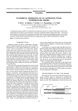
A schematic of a typical single-shielded total temperature probe with a high recovery factor is shown in Fig. 1. The high-speed, high-temperature flow crosses a bow shock in front of the probe (for the case of supersonic flow) and enters the probe, which is comprised of a sheathed thermocouple centered in a radiation shield. The shield has multiple vent, or aspiration, holes that are sized to control the flow of the gas into the probe cavity. Estimating the flow through the vents is a necessary part of the model.
The modeling efforts described in this paper have been ongoing at the University of Tennessee Space Institute for a few years. Early work towards modeling and understanding of this probe [2] has been enhanced and extended, including new CFD results are presented and compared in this paper.
DEVELOPMENT OF THE UTSI MODEL
The probe in the University of Tennessee Space Institute (UTSI) model is modeled by dividing the shield, sheath and the gas in the cavity into axial elements or cells. The temperature of each of these cells
Bow shock if supersonic
Fig. 1. Total Temperature Probe.
Gas-»-
| Insulator
I I Shield cell | Gas cell
| j T C Probe cell
| | Coolant
Fig. 2. Computational Cell Arrangement.
is determined from the relaxation of the time dependent energy equation, integrated over a cell, describing the convective, conductive, and radiative energy transport to, and between, cells. Radiation transport includes interactions with the external surroundings, as well as that inside the probe cavity. Axial symmetry is assumed in the model.
The model allows for two thermal boundary conditions at the aft end of the probe: isothermal, where the cell temperature of one or more cells at the aft end of the shield are specified and adiabatic where the axial heat flux from the aft cells is set to zero. The configuration in Fig. 2 represents an isothermal boundary condition with active radial cooling and an insulator at the base blocking the axial conduction. Aft of the vents the insulator between the probe and shield represents the actual material in this location with a finite thermal conductivity.
For the probe shield and sheath the conservation of energy for cell i is:
dT A 2T PcpV-T- = Vk AT2 + hAx(Tg - T) + dt Ax
(1)
+ hcoAx (Tg^ — Ti) — qrad,
where p is the density cp the specific heat, k the thermal conductivity, qrad the radiative flux, and h the heat transfer coefficient have an implied dependence on T and change for each cell for each time step. The term A2T/Ax2 represents the finite difference form of the partial second derivative. The term with the free stream heat transfer coefficient (hx) applies to the sheath only. The gas temperature, Tg, refers to the gas cell in contact with the surface of cell i. For both the sheath and the center body the convection term for the cells facing into the oncoming gas stream is augmented by the stagnation heat transfer.
Thermal radiation is a significant heat loss mechanism, and to assure the maximum accuracy in the calculation, radiation view factors are calculated between the cells on the radiation shield (Fig. 2) equivalent to a section of the inside surface of a cylinder to itself and other sections of the same cylinder with and without an intervening coaxial cylinder. They are also calculated between the cells on the thermocouple sheath and the shield [3, 4] equivalent to sections on concentric,
finite length, axially offset cylinders. Several approximations were made to simplify the calculation of the view factors. The hemispherical tip of the thermocouple was assumed to radiate in the forward direction only. View factors from shield cells aft of the probe tip to other shield cells were calculated as though the thermocouple extended to the entrance of the shield. All radiation (1 — l,kVi > k) coming from behind the thermocouple tip that is not collected by the sheath or shield is assumed to go to the separating insulator at the base of the cavity.
There are also view factors for external radiation from the gas to the probe cells, as well as a model for the radiation from CO2 and H2O [5]. Currently, radiation from hot surfaces in view of the probe and particles in the gas are not included in the model, although in many cases they may be significant. The view factors and material surface properties are assumed not to depend on temperature and are calculated once, prior to the solution of the temperature equations. The radiative energy exchange between the cells in the cavity formed by the inside surfaces of the shield, the surfaces of the center body cells and the cell face of the spacer (at the cavity base) looking into the cavity is calculated from the conservation of radiant energy. The radiative energy exchange balances the emitted and reflected energy from each cell and the irradiation from its neighbors. Any deviations from the assumption of a diffuse gray radiator are neglected. Openings in the cavity are assumed to be cold and black (temperature T = 0 and emissivity s = 1) and are not included in the calculation. The calculation of the radiative exchange between these cells results in a set of coupled linear equations [4]:
q - y qk(Si((i/ek) - № > i) =
4 4 (2)
= Afiia(Ti4 - y (Ft >kTk4)) - q
This set of equations is solved for the from each cell using the view factors (F), emissivities (s) for the materials in the cavity, and the current values of the cell temperatures (T). The external radiation (qx) comes from the volume of gas surrounding the probe and depends on the gas temperature and composition, as well as radiation from heated walls and engine hot parts.
In addition to the radiation from the cavity there is radiation from the external surface of the shield cells:
qi = A;spT4 - qm, (3)
where A is the cell area and a the Stephan—Boltzmann Constant.
For the gas in the probe cavity, the energy equation is:
pCpVddt~ = p"Ar(Ei-1 - Hi) + (4)
= hsAx(Ts - T) + hcAx(Tc - T),
where V is the cell volume, H the gas enthalpy, the subscript i designates the axial position of the cell, the subscripts x and r axial and radial areas and s and c the
The Effect of Perturbations on the Calculated Temperature
T probe tip [R] AT [R]/% Computational Modifications for T0 = 2500 R
2383 6/0.3 Measured [3]
2377 0/0 Baseline computation
2377 0/0 Increase shield conductivity 20%
2368 -9/-0.4 Increase thermocouple conductivity 20%
2386 9/0.4 Increase shield external heat transfer coefficient 20%
2376 -1/0 Increase shield internal heat transfer coefficient 20%
2383 6/0.3 Increase thermocouple body heat transfer coefficient 20%
2383 6/0.3 Increase thermocouple tip heat transfer coefficient 20%
2383 6/0.3 Increase the vent flow coefficient 20%
2373 -4/-0.2 Increase the thermocouple emissivity 20%
2365 -12/-0.5 Increase the shield emissivity 20%
2379 2/0.1 Include gas radiation
2371 -6/-0.3 Increase the cells in the cavity from 21 to 41
shield and centerbody temperatures in contact with the cell.
Axial conduction and radiation to or from the gas in the cavity is neglected. End
Для дальнейшего прочтения статьи необходимо приобрести полный текст. Статьи высылаются в формате PDF на указанную при оплате почту. Время доставки составляет менее 10 минут. Стоимость одной статьи — 150 рублей.