ЯДЕРНАЯ ФИЗИКА, 2004, том 67, № 3, с. 653-659
= ЭЛЕМЕНТАРНЫЕ ЧАСТИЦЫ И ПОЛЯ A NEW LOOK AT THE KLOE DATA ON THE ф ^ DECAY
© 2004 N. N. Achasov*, A. V. Kiselev**
Sobolev Institute for Mathematics, Siberian Division, Russian Academy of Sciences, Novosibirsk
Received February 4, 2003
We present the analysis of the recent high-statistical KLOE data on the ф ^ decay. This decay mainly goes through the a0Y intermediate state, what gives an opportunity to investigate properties of the a0. It is shown that KLOE data prefer a higher a0 mass and a considerably larger a0 coupling to the KK, than those obtained in the analysis of the KLOE group.
1. INTRODUCTION
The lightest scalar mesons ao(980) and /o(980), discovered more than thirty years ago, became the hard problem for the naive quark—antiquark (qq) model from the outset. Really, on the one hand, the almost exact degeneration of the masses of the isovector ao(980) and isoscalar /o(980) states revealed seemingly the structure similar to the structure of the vector p and u mesons and, on the other hand, the strong coupling of /0(980) with the KK channel pointed unambiguously to a considerable part of the strange quark pair ss in the wave function of /0(980). It was noted in late 1970s that in the MIT bag model there are light four-quark scalar states and suggested that ao(980) and /o(980) might be these states [1]. From that time ao (980) and /o(980) resonances came into beloved children of the light quark spectroscopy, see, for example, [2—4].
Ten years later there was proposed [5] to study radiative 0 decays 0 — aoj — nn°Y and 0 — /oj — — y to solve the puzzle of the lightest scalar mesons. Over the next ten years before the experiments (in 1998), this question was examined from different points of view [6—10].
Now these decays have been studied not only theoretically but also experimentally. The first measurements have been reported by the SND [11 — 14] and CMD-2 [15] Collaborations which obtain the following branching ratios:
Br(0 — Yn°v) = (8-8 ± 1.4 ± 0.9) x 10-5 [13], Br(0 — Y^V) = (12.21 ± 0.98 ± ± 0.61) x 10-5 [14], Br(0 — Yn°v) = (9.0 ± 2.4 ± 1.0) x 10-5 [15],
E-mail: achasov@math.nsc.ru
E-mail: kiselev@math.nsc.ru
Br(0 — Ynono) = (9.2 ± 0.8 ± 0.6) x 10-5 [15].
More recently the KLOE Collaboration has measured [16, 17]
Br(0 — Yn°v) = (8.51 ± 0.51 ± 0.57) x 10-5
in n — YY [16],
Br(0 — Ynon) = (7.96 ± 0.60 ± 0.40) x 10-5
in n — n+n-no [16],
Br(0 — Ynono) = (10.9 ± 0.3 ± 0.5) x 10-5 [17]
in agreement with the Novosibirsk data [13—15] but with a considerably smaller error.
In this work we present the new analysis of the recent KLOE data on the 0 — nn°Y decay [16, 18]. In contradistinction to [16], we
(1) treat the ao mass ma0 as a free parameter of the
fit;
(2) fit the phase 5 of the interference between 0 — aoY — nn°Y (signal) and 0 — pono — nnoY (background) reactions;
(3) use new, more precise experimental values of the input parameters.
All formulas for the 0 — (aoy + p°n°) — nnoY reaction taking the background into account are shown in Section 2. The results of the five different fits are presented in Section 3. A brief summary is given in Section 4.
2. THE FORMALISM OF THE 0 — aoY — nnoY AND 0 — pono — nnoY REACTIONS
In [19] was shown that the process 0 — aoy — — nn°Y dominates in the 0 — nn°Y decay (see also [5, 7], where it was predicted in four-quark model). This was confirmed in [16, 18]. Nevertheless, the main background process 0 — pno — nnoY should be taken into account also (see [16, 19]).
The amplitude of the background process fi(p) — — n0p0 — Y(q)n0(ki)n(k2) is [19]
MB = J^T^,7 n 4>akiiiPv(-&(p ~ ki)wq€ea^u^Scj€-
Dp(p — ki)
(1)
Dao (m) V (pq)
where m2 = (ki + k2)2, fia and e^ are the polarization vectors of fi meson and photon. The forms of gR(m) and g(m) = gR(m)/gRK+K- everywhere over the m region are in [5] and [20], respectively: For m < 2mK+
g(m) = x\ 1 +
2(2n) 1 — p2(m2)
P2(m|) — p2 (m2)
x arctan
1
"(1 -P2K)) -(ir + iXim^y-
(
— I arctan
\p(m2 )l
where
p(m2) = \1 —
4m
k+
\(m2) = ln
1 + p(m2) 1 — p(m2)'
m2
4n
a
1
137'
For m > 2mK+ g(m) =
2(2n)
2 glK+K- x
xl 1 +
1 — p2(m2) P2(m2(b) — p2(m2)
p(m2)(\(m2) — in) —
1
~ p(m;)(A(m;) - wr) - -(1 - p2(m|)) x
x ^(n + i\(m24>))2 — (n + i\(m ))
The mass spectrum is
dT(fi — m) drao (m)
dm
dm
+
+ rfrback(m) drint(m) dm dm
where the mass spectrum for the signal is drao(m) 2 m2T(fi — Yao,m)T(a0 — n°n,m)
a 0' dm
n
\Da0 (m)\2
According to the one-loop mechanism of the decay fi — K+K- — ja0, suggested in [5], the amplitude of the signal fi — ja0 — has the form
Ma = g(m)9^+K-9^ ((06) - , (2)
2\g(m)\2Pnn (ml — m2) ga0K+K - gaonn
3(4n)3m3d
Dn
1 Dao(m)
The mass spectrum for the background process fi — n°p — is [19]
rfrback(m) dm
where
(ml - m2)^ 128vr3m|
dxAback(m,x), (8)
i
2 glK+K- x (3)
2|p(m2)|x
Aback(m,x) = - MB\'
(9)
1
-i 4 4io 2 2 2-2 o 4 2~2 = — [rn^m^ + 2m m^m^mp — 2mr]m7Tmp —
— 2m"2 m,n m 2p + 2m4m4p — 2m2m"2 m4p + + mp m p — 2m2m"n m p + 4m"n m% m 4 +
+ mn mp + 2m 2m 6 — 2m"2 mp — 2m^ m°p +
o 4 2 2 2 2 2 2
+ m p — 2m4 mn ml — 2m2m^ m^rn p +
2 2 2 2 2 2 4 2 2 4
+ 2mnmnm^rnp — 2m m^rnp + 2mnm^rnn —
o 2 ~ 6 , 4 4 ~ 4
2m^m p + mvm^ + m^m p
94>pir9pvi
Dp(mp)
and
(4)
22 m p = m2 +
(m2 + m"2 — mln )(m| — m2)
2m2
(mi — m2)x
— (10)
m
~pnn j
pnn —
A/ (m2 — (mv — m7r)2)(m2 — (mv + m^)2) 2m
(5)
where x is the cosine of the angle between n and y momentums in the n—n° c.m. Note that there is a misprint in Eq. (6) of [19], which describes Aback(m, x): the seventh term in the brackets u+2mpmp" should be replaced by ll+mpmp'\ as above in Eq. (9). Emphasize that all evaluations in [19] were done with the correct formula.
The term of the interference between the signal and the background processes is written in the following way:
drmt(m) (ml — m2)PnV 1
(6)
dm
128n3 ml
dxAint(m,x), (11)
i
2
1
e
2
1
2
2
2
e
e
where
2
Aint(m,x) = -R ^MaM% = / m|(mp - m2v)r
(12)
= | ( (m2 - m\)m2p +
m| — m2
„ f e% gim^g^K+K-gao^jg^g^ \
I D*p(mp)Dao(rii) J'
Note that the phase 5 is not taken into account in [19]. The inverse propagator of the scalar meson R (a0 in our case), is presented in [5, 7, 21, 22]:
Dr(w) = m2R — m2 + (13)
+ ^[RenR (mR) — nR (m2)],
ab
where £ ab [RenR (mR) — nRb(m2)] = RenR(mR) — — nR(m2) takes into account the finite width corrections of the resonance which are the one-loop contribution to the self-energy of the R resonance from the two-particle intermediate ab states.
For the pseudoscalar ab mesons and ma > > mb, m > m+ one has [3, 9, 21—23]1):
nRb(m2) =
+ Pab I i + ~ In n
9Rab ~ 167T m+m-nm2 mb m — ma +
\Jm2 - 2 m2- — \Jm2 - 2 m+
m2 — - m2_ + m2 — m+
(14)
For m- < m < m+ nRb(m2) =
■ab(^2\ _ dRab 167T
m+m mb -2 ---
nm2
ma
2
- \pab(m) \ + -1pab{m) I arctan n
for m < m_
m2 m2
m2 m2
nRb(m2) =
--Pab(m) In
n
9Rab ' 167T m+m-nm2 In mb ma
\Jm+ — m2 — \Jm2_ — m2
Jm2 — m2 + m2 — m2
(16)
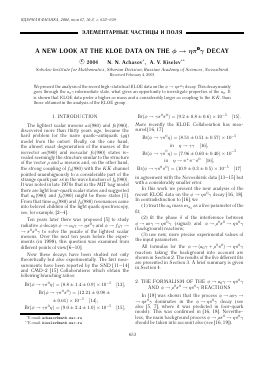
d^ nn0j)/dm, 10-4 GeV-1 6
1.0
m, GeV
Fig. 1. Plot of the fit-1 results (solid curve) and the KLOE data (points). The signal contribution and the interference term are shown with the dashed and the dotted curves, correspodingly. Cross points are omitted in fitting, the square point (0.999 GeV) is omitted in fits 3 and 4.
and
pab(m) =
1 -
m
m2
1
m
m2
(17)
m± = ma ± mb. The constants gRab are related to the width
T(R^ab,m) = -^-Pab(m).
16nm
(18)
In our case we take into account intermediate states ab = nn°, KK, and n'n0:
n
nnn0 + nK + K-
aa
+ nK °K 0 + n**
' 11ao ' ao
(19)
gaoK+K- = —gaoKoko. Note that the n'n0 contribution is of small importance due to the high threshold. Even fitting with \gaov'no \ = 0 changes the results by less than 10% of their errors. We set \gaov>no \ = = \1.13gaoK+K- \ according to the four-quark model, but this is practically the same as the two-quark model prediction ^'no \ = \1.2gaok+k- \, see [5].
The inverse propagator of the p meson has the following expression
g2 ( 4m2 \3/2 DM = m2 _ m2 _ im2 (i _ Hk ] . py ' p 48vr V m2 J
(20)
!)Note that in [21] nR(m2) differs by a real constant from those determined in other enumerated works in the case of ma = mb, but obviously it has no effect on Eq. (13).
The coupling constants g^K+K- = 4.376 ± 0.074 and g^pn = 0.814 ± 0.018 GeV-1 are taken from the new most precise measurement [24]. Note that in [16, 19] the value g^K +K- = 4.59 was obtained using
x
4
2
0
d^ n%0i)/dm, 10-4 GeV-1 5 4 3
n
0.7
0.8
0.9
dBr(^ ^ nn0y)/dm, 10-4 GeV-1 6 6
5 4 3
1.0
m, GeV
0.7
0.8
0.9
1.0
m, GeV
Fig. 2. The comparison of the fit 1 and the KLOE data. Histograms show fit-1 results averaged around each bin (see Eqs. (22), (24)) for (a) 0 ^ nn0Y, n ^ YY and (b) 0 ^ nn0Y, n ^ n+n-n0 samples.
the [25] data. The coupling constant g(„ri = 0.56 ± ± 0.05 GeV-1 is obtained from the data of [26] with the help of the expression
r(P — nY) =
g
96nm3
(m p — m2)3
(21)
i =
1
H+1
mi+i — mi
dBr(fi — nn0 Y )/dm. (22)
In this case one should define x2 function as
x2 = ^(_Blh-Bry
a:
2
(23)
where _Biexp are the experimental results, ai are the experimental errors, and
rrii+1
Bth =
1
dBrth(fi — nn0Y)/dm (24)
mi+i — m.
3. RESULTS
The KLOE data on the fi — nn°Y decay may be found in Table 5 of [18] (see also Figs. 1, 2). The data is separated into two samples: the first consists of events in which n decays into 2y, while events in which n decays into 3n correspond to the second sample, see Fig. 2. Note that as in [16, 18], we do not fit 1 st, 10th, and 27th points of this table (cross points in the Fig. 1). Emphasize that the 10th (1.014 GeV) and 27th (1.019 GeV) points are obvious artifacts because the mass spectrum behavior on the right slope of the resonance has the form (photon energy) 3 according to gauge invariance.
In the experiment the whole mass region (mn + + mno,mi) is divided into some number of bins. Experimenters measure the average value Bi ("i" is the number of bin) of
Для дальнейшего прочтения статьи необходимо приобрести полный текст. Статьи высылаются в формате PDF на указанную при оплате почту. Время доставки составляет менее 10 минут. Стоимость одной статьи — 150 рублей.