- (1 - 2^)dx2 - dxidxj(hij)]
used in order to formulate the cosmological perturbation theory [1] leads to questions:
(i) What is the difference between the coordinate evolution parameter x0 in the Hamiltonian approach (3) and the conformal time n in Lifshitz's theory (5)?
(ii) What is number of variables (in particular, homogeneous ones) in GR?
(iii) What is difference between potentials ^ and variables Nd,
3. THE DIFFEO-INVARIANT HAMILTONIAN APPROACH
The forms (4) are invariant with respect to the kinemetric general coordinate transformations x0 ^ ^ x0 = p0(x0), x1 ^ xi = xi(x0,xl) [8]. This group of diffeomorphisms of the frame (4) means that the coordinate parameter x0 is not observable. One of the main problems of the Hamiltonian approach to GR is to pick out a diffeo-invariant global variable which can be evolution parameter. There is a set of arguments [6, 7, 10] to identify this evolution parameter in GR with the cosmological scale factor a(x0) introduced by the scale transformation: F (") =
= an(x0)F(n), where (n) is the conformal weight of any field, including metric components, in particular,
_ _2
the lapse function Nd = a-2Nd and ^2 = a.
The transformation of a curvature \/-gR(g) = = a2\/—§R(g) — 6acj0[cj0ay/—gg°0] converts action (1) into
5 [^0] = S M -J dx0 W J = j dx°C,
Nd (6)
where S[p] is the action (1) in terms of metrics g, p(x0) = p0a(x0) is the running scale of all masses of the matter fields, and (Nd)-1 = \/-gg00.
The energy constraint 5S[p0]/5Nd = 0 takes the algebraic form [6]:
M _ To _
W - To =
(M2 n 2
(7)
where Tq is the local energy density. The spatial averaging of the square root of this equation
i d3xJT_
s*x -WT«7 = ^KtJ = (8)
= ± I = *
has the exact solution in the form
fo
( (,0b) -j = ±j-
dip
(VToW)Y
where Z is a diffeo-invariant time, if the local density T0 does not depend on the velocity p'. The substitution of this solution in (8) determines the diffeo-invariant local part of the Dirac lapse function:
((Nd)-1)Nd =
vn
(10)
The diffeo-invariant evolution (9) can be treated as the GR analogy of the Hubble law in a cosmological model considered in the lowest order of the cosmological perturbation theory T0 ~ p0(p), Nd = N0(x°), where the Hilbert action (1) and the interval of the diffeo-invariant time Z take the form
^Wheeler—DeWitt = (11)
= Vo dx No
{N^o)2 + po(b)
Z = J Nodx0.
This form keeps the symmetry of GR in the homogeneous approximation x0 — X0 = X0(x0), N0 = = N0dx°/dx°. One can see that the diffeo-invariant time Z coincides with the conformal one.
In the Hamiltonian approach, the action (11) takes the form
5 = dxo
No
4Vo'
-Pfdob + 7To(Pf - K)
where Ev = 2V0^/p0 is treated as the reduced energy, since the scale factor p plays the role of evolution parameter; whereas the canonical momentum Pv is considered as the reduced Hamiltonian function. It is a generator of the evolution with respect to the scale factor p forward, or backward in the Wheeler— DeWitt (WDW) field space of events depending on a sign of resolution of the energy constraint P^ — E2 = = 0 — Pv± = ±E^. The problem of the negative reduced energy (defined as values of the reduced Hamiltonian function onto equations of motion) is solved by the primary and secondary quantizations of the energy constraint in accordance with QFT confirmed by high-energy physics experiments.
The primary quantization is known in Quantum Cosmology as the WDW equation [11]: —
— E2]^wdw = 0, here Pv = —id/dp (or d2^wdw + + E2^wdw = 0). In order to diagonalize the
WDW field Hamiltonian, this equation is rewritten in terms of holomorphic variables [5] ^WDW = = (1/^2EV)[A+ + A-], where A+, A- is the operators of creation and annihilation of a quant of a universe (this quant can be called a "wheeleron") after the secondary quantization of the WDW field.
The Bogoliubov transformation: A+ = aB + + + 3*Bdiagonalizes the equations of motion
by the condensation of wheelerons ( 0
2 -
0 ) = R(p) and describe cosmological
dp
dR(<p)
dp
2Ef dp
= -2EV\/4N(N + 1) - R2.
(13)
In particular, in the model of the stiff (rigid) state p = p, where Ev = Q/p, the Bogoliubov equations (12) and (13) have an exact solution, as N =
J- R-
4Q R:
N (p) =
1
4Q2 - 1
sin
Q2 - 1 in p
4 pi
= 0,
(14)
where
p = pi^J 1 + 2Hi n
d3x[log^ - (log= 0.
(16)
One can construct the Hamiltonian function using the definition of a set of the canonical momenta:
P = _ dL f d(dop)
= 2Vop',
(17)
P^
dL _ 4p2 d^N1) - o>o(/)
d(do log
/ N d
-A-A-]
creation of a "number" of universes as wheelerons (0|A+A-10) = N(p) from the stable Bogoliubov vacuum B-l0) =0 [12]. Vacuum postulate B-l0) = = 0 leads to an arrow of the conformal time n > 0 and its absolute point of reference n = 0 at the moment of creation p = pI [6, 7].
Cosmological creation of the "universes'" is described by the Bogoliubov equations
4NN + 1)- ^ (12)
(18)
Now, using solution (10) and definitions (17), (18) one can express action in the Hamiltonian form in terms of momenta Pv and PF = p,,p(a),pf]
S[po] = y dx0 J d3x ^^ PfdoF + cj - (19)
P2 - E2
- Pvdop + f f
4 J dx3(Nd)
where the reduced Hamiltonian function
73 „
Ev = 2 J d3x^JT0 = 2Vo^y/T^
(20)
can be treated as the "universe energy" by analogy with the "particle energy" in special relativity (SR), and C = NiT0 + C0p^ + C(a) dke\a) is the sum of constraints with the Lagrangian multipliers Ni,C0, C(a) and the energy—momentum tensor components T0; these constraints include the transversality die(a) — 0 and the Dirac minimal surface [3]:
p^ ^ 0
d3 (/N ) = (/)'
(21)
(15)
and the initial data pI = p(n = 0), HI = p'I/pI = = Q/(2V0p?) are considered as a point of creation or annihilation of a universe; whereas the Planck value of the running mass scale p0 = p(n = no) belongs to the present day moment no, and the so-called Planck epoch connecting the present-day value of the evolution parameter p0 with the initial data becomes very doubtful.
4. NUMBER OF VARIABLES AND CONSTRAINTS In order to keep the number of variables of GR, the scale factor can be defined using the spatial averaging log^ = (log so that there is the identity
(Nj = Nj (N-1 )),
where p^ is defined by (18). One can find evolution of all field variables F(p, xi) with respect to p by the variation of the "reduced" action obtained as values of the Hamiltonian form of initial action (19) onto the energy constraint P? = E? [6]:
]\PV=±EV =
(22)
fo
= / dp
d3 x
Y^Pf dv F + C
F
where C = C/d0p. The reduced Hamiltonian Vr0 is Hermitian as the minimal surface constraint (21) removes negative contribution of p^ from energy density. Thus, the diffeo-invariance gives us the solution
3
of the energy problem in GR by the Hamiltonian reduction like solution of the similar problem in SR.
The explicit dependence of T0 on ф was given by Lichnerowicz [13] by extracting the Laplace operator
ДF = ^d(b)d(b)F: T0 = ф7Дф + ЕФti, where ti is partial energy density marked by the index I running a set of values I = 0 (stiff), 4 (radiation), 6 (mass), 8 (curvature), 12 (Л term) in the correspondence with a type of matter field contributions.
5. THE DIFFEO-INVARIANT PERTURBATION THEORY
Let us introduce a parametrization of metric \-i
(Nd) 1 ,ф through functions ß, v
(N d)
1
((N d)-1)
= 1 + v,
ф = e»
(23)
with the zero spatial "averaging" (16) fx = fx and v = = v. These functions are determined by the equation
öß
= (1 + v )
1
Ie»I ti + 7e7»Â ■ e»
+ e»Â ■ [e7»(1 + v)-1] =0
(24)
and the energy constraint (10) 1 + v =
where T00 takes form
(\TY
T0 = eT»A e» + Y e»1 ti ,
(25)
(26)
2(t(o) )
The first order of (24) T(1) + ((t(2)) + 14A) • f — — ((t(1)) + A) • v = 0 gives v and fx in the form of sum of the Green functions [D(±) • J(±)](x) =
= / d3 yD(±)(x,y)J(±) (y):
ß = 14в D+) ^ J(+) " D(-) ^ J(-)]
1
where 3 = j 1 + [(t{?)) — 14(t{v) )]/(98(t(o) )),
J(±) =7(1 ± 3)t(0) — t(1) are the local currents, D(±) are the Green functions satisfying equations
(31)
[±m2±) - A]D(±)(x,y) = ö3(x - y), m2±) = 14(в ± 1)(t(O))^(T(I)).
(32)
TI = (ti ) + TI, (ti ) = 0.
and each partial energy density ti is a sum of the "averaging" one (ti) and the "deviation" (16) ti = = ti — (ti). The Dirac constraint of minimal surface (21) takes the form d(b) (e6ßN(b)) = dc(e62). The diffeo-invariant perturbation theory can be defined as a power series in ß, v, and "deviations" of densities ti:
TO = To + Ti + T2 + ..., (27)
where To = (t(o) ), Ti = T(o) + ((T(i)) + A) • ß, T2 = ß T(i) + ((t(2) ) + 14AA) • 2] + iA • ß2, and T(n) = £ inTi. In the first order, (25) takes a form where
I
1 + v = 1 + Tl = 1 + iss + ((T(1)) + A) •ß 2T0
In the case of point mass distribution in a finite volume V0 with the zero pressure and the density T(1) = = t(2) /6 = £ Mj[53(x — yj) — I/V0], solutions (29),
J
(30) take the very significant form:
f(x) = Y}rgj/(4rJ )H7i e-mM(z)rj + (33) j
+ (1 — 71) cos (m(-)(z)rj)], v (x) = ^[2rflj/rj ][(1 — 72)e-m(+)(z)rj + (34)
+ 72 cos (m(-) (z)rj)],
Yi
1 + 7 в 14ß ,
72
(1 - ß)(7ß - 1) 16 ß :
(28)
3Mj
rJ = ^, rJ = Iх - yJ\.
The minimal surface (21) di[^> Ni] — C06)' = 0 gives the shift of the coordinate origin in the process of evolution:
n* = ( 'xn (9<V
(29)
r ) V dr V
r
V(C,r) = J dr T2e6»(z'rr.
v = 2в ^ + в)D(+) ^ J(+) - (1 - ß)D(-) ^ J,
(30)
(35)
In the infinite volume limit (T(n) ) = 0 these solutions take the standard Newtonian form: fx = D • T(0),
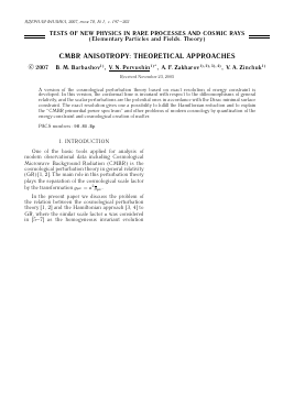
Nz (x) 0.06
25 0 T
Longitudinal (NZ(x)) components of the boson distribution vs. the dimensionless time t = 2^HI and the dimensionless momentum x = q/Mi at the initial data Mi = Hi .
v = D • [14t(0) — t(1) ], Ni = 0 (where AD(x) = in the space determined by the interval = —53 (x)).
6. APPLICATIONS
The reduced action (22) determines evolution of fields directly in terms of the cosmological scale factor a = f/f0 connected with the redshift parameter z by the relation f = f0 / (1 + z).
Let us propose that the homogeneous density {t(u)) = P(n) (
Для дальнейшего прочтения статьи необходимо приобрести полный текст. Статьи высылаются в формате PDF на указанную при оплате почту. Время доставки составляет менее 10 минут. Стоимость одной статьи — 150 рублей.