Pis'ma v ZhETF, vol. 97, iss. 8, pp. 529-535 © 2013 April 25
Non-stationary regimes of surface gravity wave turbulence
R.Bedard, S. LukaschukS. Nazarenko+ Department of Engineering, University of Hull, Hull, HU6 7RX, UK + Mathematics Institute, University of Warwick, Coventry, CV4 7AL, UK
Submitted 26 February 2013 Resubmitted 27 March 2013
We present experimental results about rising and decaying gravity wave turbulence in a large laboratory flume. We consider the time evolution of the wave energy spectral components in u- and fc-domains and demonstrate that emerging wave turbulence can be characterized by two time scales - a short dynamical scale due to nonlinear wave interactions and a longer kinetic time scale characterising formation of a stationary wave energy spectrum. In the decay regime we observed the maximum of the wave energy spectrum decreasing in time initially as the power law, a: t-1/2, as predicted by the weak turbulence theory, and then exponentially due to viscous friction.
DOI: 10.7868/S0370274X13080055
Surface gravity waves generated by wind represent a practically important and most studied example of wave turbulence. Such waves are of small amplitude in most natural cases and can be described by a weak turbulence theory (WTT) [1]. A small parameter is the ratio of the wave height to its length n/\ C 1 or the wave steepness kn, where k = 2n/\ is the wave vector. The WTT considers statistics of isotropic ensembles of dispersive weakly nonlinear interactive waves and predicts a scale invariant form of the wave energy spectra Ek « k-^ and « within the universal interval (kf ,kd). Here w is the wave frequency, the subscripts f and d are related to the forcing and dissipative scales respectively. It is assumed that kd ^ kf. For isotropic surface gravity wave turbulence the WTT predictions for the spectral exponents are n = 7/2, v = 4 known as Kolmogorov-Zakharov (K-Z) spectrum.
K-Z spectrum was confirmed numerically in [2], though within less than a decade universal interval. The most advanced field experiments done by Hwang et al. [3] show the energy spectra exponents close to the WTT predictions, though the wave fields in that experiment were not isotropic and near surface wind was not measured. Incomplete knowledge of external factors such as wind, currents and various gradients of physical parameters makes interpretations of the field experiments difficult. Parameters of laboratory experiments are under much better control and some small scale experiments with capillary wave turbulence demonstrate good agreement of measured v-exponents with the WTT pre-
1)e-mail: S.Lukaschuk@hull.ac.uk
dictions, see for example [4]. In our recent experiments with gravity waves in a large flume [5, 6] we observed dependence of the v- and ^-exponents from the averaged wave amplitude or the coefficient of wave nonlin-earity 7 = kf^J(i]2(t, r)}, where (...) denotes mean taken over the time or space. We explained this dependence as a result of three possible mechanisms [7]: four-wave interactions, finite size effects and wave breaking. Our measured exponents asymptotically approach the values predicted by the WTT at large wave amplitudes with Y « 0.25, where apparently that theory should not be applied.
Most of the previous laboratory studies of wave turbulence were concerned with statistics of stationary regimes. Just a few experiments dealt with non-stationary cases and all of them are about the decay of capillary wave turbulence [8, 9]. As far as we are aware, characteristics of non-stationary gravity wave turbulence had never been studied experimentally. This paper presents our new experimental observations of rising and decaying regimes of gravity wave turbulence and their analysis in terms of temporal evolutions of the energy spectral modes in w- and fc-domains. For the first time we present here the measured characteristic time for wave turbulence formation and observations of a non-monotonic character of the spectral mode decay at the intermediate scales within the universal interval.
There are two time scales which will be useful for our further discussion. The dynamical scale td is the characteristic time of deterministic nonlinear dynamical equations for surface gravity waves. It can be derived from a knowledge that the leading order wave interac-
tion process for surface gravity waves is four-wave and therefore n1 K V2V3V4- It follows from here that the dynamical time is inversely proportional to the square of the wave amplitude. The rest of the expression can be reconstructed from dimensionality by adding the wave frequency w and the gravity constant g:
td
g
w5n2
(1)
The kinetic time scale can be obtained from the dimensional analysis of the kinetic equation [1] based on the fact that, the inverse characteristic time must be proportional to the fourth power of the wave amplitude and the rest is reconstructed dimensionally:
tk
g
2 -2 V„A=TDUJ = 1 tD-
(2)
For our typical experiment n ~ 5 cm, w ~ wf = 2nf, where f is the forcing frequency which is about 1 Hz. We have the nonlinearity parameter y ~ 0.2, td ~ 4 s and tk ~ 100 s. Note that the timescales are very sensitive to the values of n and wf. Once the forcing is switched off the kinetic time rapidly increases due to the strong dependence of tk on n.
Let us suppose that the kinetic equation of weak wave turbulence is valid from the very first moment after the pumping of energy is turned on, and consider formation of the steady state spectrum. There are several types of self-similar evolution. To identify one for gravity waves we notice that this is a finite capacity system, i.e. only a finite amount of wave energy is necessary to fill up the high-frequency tail of the K-Z-spectrum for whatever large inertial intervals. Thus, no matter how high the dissipation frequency is, the propagating front of the spectrum will reach from the forcing to the dissipation frequency in a finite time which is of an order of the kinetic characteristic time Tk (2). It is interesting that the spectrum left behind a propagating front is steeper than the K-Z-spectrum. The K-Z-spectrum will finally form as a reflection wave propagating toward lower frequencies after the front hits the high-frequency end of the inertial range [10, 11].
We obtain an estimation of characteristic time for decaying wave turbulence from the kinetic equation which describes the stationary wave turbulence regime. Again, due to the finite system capacity, only a small amount of energy supply is necessary to maintain the K-Z-spectrum. In the decaying stage this supply is provided by the lowest frequencies containing most of the energy. Thus, in the decaying stage we should expect the K-Z-spectrum in the inertial range whose overall amplitude is gradually decreasing as the energy is slowly leaking from the system. Because most of the wave energy
resides near the forcing frequency wf , the wave energy density per unit area of the water surface E can be estimated as EU{ as E = fuf Eu dw ~ EU{ wf. Thus, for
the energy dissipation rate e = —E ~ —EUf wf. Substituting e from the K-Z-spectrum taken at wf, we have
E
-e/uf — -Et g
3 ~-6f
This gives
Ef —
11/2
-1/2
(3)
(4)
Thus according to the weak turbulence theory the peak of the energy spectrum should decay as an inverse square root of time.
Finally, let us estimate characteristic time of linear dissipation occurring at the lateral walls of the flume. Linear dissipation on the walls becomes dominant at smaller wave amplitudes. The estimate could be made based on the well-known textbook problem about the oscillating laminar flow with velocity amplitude u and frequency uj near a flat boundary. This layer has an exponential velocity profile with thickness S ~ ^/2v/uj and, therefore, the energy dissipation rate in this layer is 2v5~2u2V ~ wu2V, where V = 4LSH is the total volume of the boundary layer, with L being the flume size and H ~ g/w2 being the characteristic depth of the wave motion. Dividing the energy dissipation rate in the layer by the total wave energy u2L2H, we get the exponent of the exponential decay of the wave energy due to the wall friction:
L '
(5)
Substituting here v = 10-6 m2/s, w — Wf = 2n s-1 (1Hz forcing) and L — 10 m, we get av — 1/1000 s-1.
In addition we can estimate the amplitude corresponding to the crossover from the dominant cascade to the friction dissipation mechanism. It occurs when tkav — 1, which, taking into account (2), gives nc — 3 cm. Thus we see that when the wave amplitudes will reach to just 3 cm we should expect that the cascade dominated dissipation of energy should be replaced by the wall friction mechanism. For the crossover time we have tc — tK ln(5/3) — 500 s. Because of the singular character of the t-1/2 law at t = 0, the crossover time is almost insensitive to the initial wave intensity.
Experimental procedures. Our experimental setup was the same as described in [7]. The flume with dimensions 12 x 6 x 1.5 m3 was filled with water up to the depth of 0.9 m. The gravity waves were excited by a piston-type wave maker consisting of 8 separate sections covering the short side of the flume. The wave
3
g
t
4
a,, ~
V
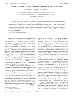
1 Hz filter 3 Hz filter 5 Hz filter 7 Hz filter
Mean stat. amplitude
1200
Fig. 1. The time evolution of the band passed filtered wave amplitudes in the rising wave turbulence regime for the record with y = 0.25. Filter frequencies are equal to 1, 3, 5, 7 Hz. The bandwidth of 1 Hz is the same for all frequencies. Dashed lines show the averaged levels of filtered amplitudes in the stationary stage
maker generated a superposition of two waves of equal amplitudes and with frequencies fi = 0.993 Hz and f2 = 1.14 Hz (the wavelengths are 1.58 and 1.2 m correspondingly). The wave vector ki was perpendicular to the plane of the wave maker and k2 was at the angle 9° to ki. The dissipation for one-meter waves is sufficiently low and the waves undergo m
Для дальнейшего прочтения статьи необходимо приобрести полный текст. Статьи высылаются в формате PDF на указанную при оплате почту. Время доставки составляет менее 10 минут. Стоимость одной статьи — 150 рублей.