ТЕОРЕТИЧЕСКИЕ ОСНОВЫ ХИМИЧЕСКОЙ ТЕХНОЛОГИИ, 2014, том 48, № 5, с. 538-550
УДК 66.011
PARAMETER IDENTIFICATION FOR ORDINARY AND DELAY DIFFERENTIAL
EQUATIONS BY USING FLAT INPUTS © 2014 René Schenkendorf, Michael Mangold
Max Planck Institute for Dynamics of Complex Technical Systems Sandtorstrafie 1, 39106 Magdeburg, Germany mangold@mpi-magdeburg.mpg.de Received 01.04.2014
The concept of differential flatness has been widely used for nonlinear controller design. In this contribution, it is shown that flatness may also be a very useful property for parameter identification. An identification method based on flat inputs is introduced. The treatment of noisy measurements and the extension of the method to delay differential equations are discussed. The method is illustrated by two case studies: the well-known FitzHugh—Nagumo equations and a virus replication model with delays.
Keywords: mathematical models, parameter identification, ordinary differential equations (ODE), delay differential equations (DDE), flat inputs, differential flatness, differentially flat systems.
DOI: 10.7868/S0040357114050091
INTRODUCTION
Virtually all mathematical models of chemical or biochemical processes contain unknown parameters that have to be identified from experimental data. Parameter identification is therefore a central step during the development of mathematical models and a prerequisite for model based process control and process design.
In most cases, parameters are identified from experiments as shown in Figure 1a, see e.g. [1]. A process
model E is set up to reproduce the experiments in simulations, using the operation conditions or inputs u as
in reality and an estimate 0 of the unknown model parameters 9. In most cases, this requires a numerical solution of the differential equations of the model. The simulated process output or measurement y is then compared to the true output y. If there are deviations, the estimate of the parameters is refined iteratively in an optimization step. Nowadays, the numerical solution of differential or differential algebraic systems is usually not very challenging, but it may become tricky when the guesses of the parameter values or of unknown initial conditions are poor and far away from the true values. Problems arise especially, when the system equations contain delay terms, because then initial functions over a delay interval before the experiment's starting time have to be estimated and because the numerical solution of delay differential equations in general is more difficult. Further, numerical integration underlying an optimization procedure may be quite expensive and consume the biggest share of the
spent computation time. Finally, the dependence of the system outputs on the model parameters is often strongly nonlinear, resulting in non-convex cost functions with local minima for parameter identification. The mentioned difficulties motivate the search for alternative approaches for parameter identification.
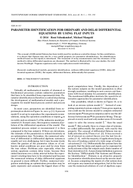
One possibility, which is shown in Figure 1b, is to look at an inverse system model 2-1. Instead of computing simulated system outputs y from given inputs u, one could use the inverse model to compute estimated system inputs U from given outputs y and to use the difference between u and U for parameter fitting. This approach is rarely used and only makes sense if it is much
easier to solve the inverse model £-1 than the usual
model £. But actually, there is a large class of systems, so-called differentially flat systems, with exactly this property. The concept of differential flatness was initially introduced by Fliess et al. [2]. It has received a lot of interest in control theory over the last two decades [3, 4], with the majority of applications lying in the area of tracking control of a wide range of technical systems [5—11]. Differentially flat systems have the property that the states and inputs can be expressed directly in terms of the flat outputs and a finite number of their derivatives [12]. A more formal definition is given in the Section "Differentially Flat Systems and Parameter Identification". Flatness is an attractive property for parameter identification based on the inverse model, because computing the inputs of a flat system does not require any numerical integration, but in the worst case the numerical solution of a set of algebraic equa-
PARAMETER IDENTIFICATION FOR ORDINARY AND DELAY DIFFERENTIAL EQUATIONS 539 (a) (b)
Х(в) SO)
-> y u >
Ш X 1(у)
У u
У
u
Fig. 1. Alternative approaches for parameter identification: (a) by fitting a simulated system output y to the measurements y; (b) by fitting a reconstructed input u to the true input u using an inverse process model.
tions. The topic of this paper is to study the use of flat inputs for parameter identification. Flat inputs mean input variables that turn given outputs to flat outputs and hence enable a differential parametrization of the model [13].
Vassilev et al. [14] exploited flatness properties of a precipitation reaction model in order to identify a single physical model parameter, which is hardly accessible to direct measurements. They made use of the fact that in their case the unknown parameter happens to be a flat input of the system and obtained convincing estimation results for that parameter. The drawback of the method by Vassilev et al. is that it requires a very special model structure and that it requires as many measurement variables as there are unknown parameters, whereas the flat input method presented here is applicable to a much larger class of systems.
A related identification method was introduced by Fliess et al. [15] for systems, whose parameters can be expressed by algebraic equations depending on the inputs, the outputs and time derivatives of both. The charm of this method is that it does not require any numerical optimization, but only the solution of an algebraic set of equations, and hence is very fast. As a disadvantage, it may require a high number of derivatives of inputs and outputs, if the number of unknown parameters is large compared to the number of inputs and outputs.
The flat input method has similarities to methods of functional data analysis and principal differential analysis (PDA). Early publications in that field [16, 17] assume all model states to be measurable. The states are approximated by splines or similar functions and fitted to the measurements, introducing "nuisance" parameters in addition to the model parameters. The residuals resulting from inserting the state approximations into the differential equations of the model are minimized in order to obtain estimates of the model parameters. Over the years, the method has been more and more refined in order to cope with measurement imperfections and increase accuracy [18—24]. Powerful techniques of iterated and cascaded parameter estimation approaches have been developed in this context, which also prove to be useful for the flat input approach. The main difference, however, is that in PDA all states are parametrized independently, resulting in
a quite large number of nuisance parameters, and that the technique is mainly used for systems that have hardly hidden unmeasured states. In contrast, the flat input method only introduces nuisance parameters for the measured outputs — internal system states and inputs are then automatically parametrized, as well. This reduces the number of parameters to be identified especially for systems with many unmeasured states. Another difference between PDA and the flat input method is that in this work system inputs are reconstructed. The deviations of the reconstructed inputs from the true inputs are taken as an indicator for the quality of the parameter estimate and enter the cost function for optimization.
The flat input method for parameter identification also bears some similarity to the method of differential elimination [25—29]. Differential elimination uses the theory of Grobner bases to eliminate unobserved variables from systems of differential equations that can be expressed as differential polynomials. It has been applied successfully to the estimation of parameters [25, 26] as well as to determine global identifiability of model parameters [27, 29]. Differential elimination requires reaction kinetics with certain structures (polynomial or fractional expressions), because the model equations are solved analytically for the unobserved variables. This is a difference to the flat input method that only requires implicit algebraic equations for the states and system inputs and hence is applicable to a wider class of systems.
The Section "Method" of this paper presents the method of flat inputs for parameter identification of differential equations with or without delays. The Section "Case Studies" illustrates the properties of the method by two case studies.
METHOD
The next section gives a brief introduction to differentially flat systems and to the proposed identification method. The Section "Determination of Flat Inputs" addresses the problem of how to find (potentially fictitious) inputs that turn a system into a flat system. The Section "Treatment of Measurement Noise" contains the treatment of noisy measurements in the context of the new identification method. The extension of the
method to systems with delay is discussed in the Section "Treatment of Systems with Delay".
Differentially Flat Systems and Parameter Identification. This work mainly concerns input-affine systems of the following type:
x(t) = f (x(t), t, 0) + ¿y,(x(0,0)u(t); x
(1)
i=1
where x(t)is the state vector, u(t) = (ub...,um) is the input vector, and 9 is a vector of constant model parameters. A system of type (1) is called a differentially flat system, if the following conditions hold [2, 5, 12]:
1. There is a so-called flat output y(t) = (y1(t), ...,
ym(t) that can be calculated from the state x(t), the input u(t), and t
Для дальнейшего прочтения статьи необходимо приобрести полный текст. Статьи высылаются в формате PDF на указанную при оплате почту. Время доставки составляет менее 10 минут. Стоимость одной статьи — 150 рублей.