Július Bems, Oldnch Stary Smart Bankruptcy Prediction Modelling. Artificial Intelligence Approach
Smart Bankruptcy Prediction Modelling Artificial Intelligence Approach
Július Bems,
Ing., Dept. of Economics, Management and Humanities, Faculty of Electrical Engineering, Czech Technical University (инженер, отдел экономики, менеджмента и гуманитарных наук, факультет электротехники, Чешский технический университет) (Technická 2, 166 27 Prague, Czech Republic; e-mail: bemsjuli@fel.cvut.cz)
Oldrich Stary,
CSc., prof. Ing., Dept. of Economics, Management and Humanities, Faculty of Electrical Engineering, Czech Technical University (кандидат наук, профессор, отдел экономики, менеджмента и гуманитарных наук, факультет электротехники, Чешский технический университет) (Technická 2, 166 27 Prague, Czech Republic; e-mail: bemsjuli@fel.cvut.cz)
Аннотация. В статье предложен инновационный подход к моделированию прогнозирования банкротства. Главная идея - использование измененной диаграммы паука в оценке условий компании и обеспечение регрессионного анализа по этой оценке. Параметры измененных диаграмм паука и параметры регресса оцениваются стандартным статистическим методом, а также методом искусственного интеллекта. Основной результат статьи - методология прогноза компании, который может дать нам относительное сравнение компаний и способ оценить критическое значение, выше которого компания не выполнит своих обязательств.
Abstract. This paper is covering the innovative approach of bankruptcy prediction modeling. The main idea is using modified spider diagram in assessing company conditions and providing regression analysis over this assessment. The parameters of modified spider diagrams and the parameters of regression will be estimated using standard statistical method as well as artificial intelligence methods. The major output of this paper will be methodology of company default forecast, which can provide us relative comparison of companies and the way to estimate the critical value above which the company is likely to default.
Ключевые слова: банкротство, прогнозирование, диаграмма паука, регресс, искусственный интеллект.
Keywords: bankruptcy, prediction, spider diagram, regression, artificial intelligence.
Introduction
Default forecasting (or credit scoring methods) started to be widely developed in the 60's of the last century. The pioneer in this field was Edward Altman, who developed statistical model for prediction company probability in two years. He took several accounting ratios calculated from financial statements and developed model based on linear discriminant analysis. The results was the linear combination of ratios and final score. The main idea of default prediction model is the same also nowadays. Mostly used is logistic regression approach, which has advantage of output in 0 - 1 interval, that represents probability. Logistic regression uses transformation of linear combination to logistic function. Final model is optimized by maximum likehood method, which does not have analytical solution, so numerical approach have to be used. Logistic regression and other non-linear and artificial intelligence methods started to be popular with expansion of computers since late 80's.
The main idea of this article is to integrate spider diagram area calculation with artificial intelligence methods to develop new type of regression model. Inspiration in using of spider diagram is Kaldor's Magic Square. It is the kind of spider diagram with four perpendicular axes, where each axis represents macroeconomic indicator. The higher the
area of square means better economic condition of monitored country. The same approach will be applied for companies.
Proposed Methodology
Data samples
For model development, it is necessary to have at least two sets of data: training sample and testing sample. Training sample is usually 70-80 % of data and rest is used for testing. Another option is to use cross-validation method, where training and testing sets are dynamically changing. For model validation is used another set of data, usually gathered later than training and testing set. Validation data are used to prove model performance.
Variables selection
The initial part of model development includes variables selection. Each variable is tested for its performance by several test of which the most important is the correlation between variable value and observed output. In our case, observed output is information about company bankruptcy (default). Another important variable usability test is rank ordering performance (ROPM), which is represented by relative operating characteristic (ROC) curve, cumulative accuracy profile (CAP) curve and GINI coefficient. This test will be explained in more details in Models Evaluation section. In ideal case,
Экономика и предпринимательство, № 6, 2O14 г.
МИКРОЭКОНОМИКА
default should be linearly dependent on variable value. It means, that higher (or lower) variable value leads to lower default rate. In other words, higher (or lower) is better. It this condition is not met, variable specific transformation can be made. Variable can be also divided into several group with values respecting linear dependency of default on group values.
When useful variables from previous step are selected, it is necessary to test for correlation between each other. Two or more variables with high correlation are not needed to be included in model. It is enough to use only one of them.
Models evaluation
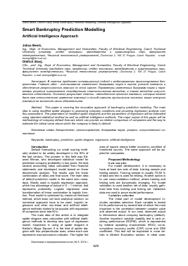
Model discrimination ability is evaluated by two main quantitative characteristics, GINI coefficient and Kolmogorov-Smirnov coefficient, and qualitative characteristics such as ROC and CAP curve shape. The Figure 1 depicts the CAP curve. Horizontal axis represents cumulated ordered population rate and vertical axis represents cumulative observed value rate, in our case company default. All companies are ordered by computed default probability. According to Figure 1 one can say that in the 15 % of population ordered descending order by default probability, 60 % of defaulted companies occurs. The blue line shows performance for companies ordered by model outputs, orange line represents random ordering and the grey line shows ideal ranking where all defaulted companies have highest default probabilities. Accuracy ratio or GINI coefficient is the ratio between area A and A + B, where A is the area surrounded by the blue and orange line and B is the area surrounded by the blue and grey line.
100% 90% 80% 70% 60% 50% 40% 30% 20% 10% 0%
85296307418529 1223455677899
Figure 1: Example of CAP curve.
Horizontal axis represents cumulative ordered population rate.
Vertical axes represents cumulative default
rate
Figure 2: Example of ROC curve
Horizontal axis represents cumulative non-default rate
Vertical axis represents cumulative default rate
The Figure 2 shows ROC curve. The difference between ROC curve and CAP curve is in horizontal axes, where in case of ROC curve the cumulative non-default rate is used instead of whole population. The better model is, the higher area under ROC curve (AUROC) is. The simplest explanation of GINI coefficient based on ROC curve is:
GINI = 2x AUROC -1
(1)
GINI coefficient value range is <-100 %; + 100 %>. Value of 100 % represents ideal or best model and 0 means random ordering of default and non-default events. Negative values mean worse than random ordering, which is mostly caused by reverse ordering.
100% 90% 80% 70% 60% 50% 40% 30% 20% 10% 0%
85296307418529
Figure 3: Kolmogorov-Smirnov curve
Journal of Economy and entrepreneurship, Vol. 8, Nom. 6
Julius Bems, Oldnch Stary Smart Bankruptcy Prediction Modelling. Artificial Intelligence Approach
Kolmogorov-Smirnov curve, the grey line from Figure 3, represents difference between non-default (good) and default (bad) rate. The maximum value of this curve is called Kolmogorov-Smirnov value.
The curves shape is also very important for model assessment. Despite high GINI value, the blue line from Figure 1 should never cross diagonal line or randomly ordered observations. The line should be concave and smooth.
Model
The most suitable variables selected by methods described in previous sections, will enter the final model. Variable values will be depicted in the spider diagram chart. The main investigated characteristics of the diagram will be spider diagram area and amount of convexities of this diagram. Companies with higher diagram area and minimal amount of convexities, should be rated better than companies with low area and higher count of convexities. Output characteristics of spider diagram are dependent on variable order, angle between variable axes and variable weight, which is represented by the axis length.
variables.
Variables values will be transformed to the interval between 0 and 1. Values with positive impact will have higher value than values with negative impact.
The outcome of this methodology is the model, which can be used for company assessment. Model input consists of transformed variables values and information concerning to convexities. Angles between axes, variable order and variables weights will be adjustable parameters. Neural networks, support vector machines, gradient descent and other methods can be used to find out the suitable configuration. Neural networks will be preferred in
our research due their popularity, scalability and suitability in regression based tasks.
In the first, learning stage, the development set of observations will be used. Neural network will get information about results. In other words, this network will adjust available parameters to get closest to known results. Then the testing and validation phase will be provided according to procedures described in models evaluation section. Results of artificial intelligence methods will be continuously compared to widely used logistic regression approach.
The most essential output of model will be the pro
Для дальнейшего прочтения статьи необходимо приобрести полный текст. Статьи высылаются в формате PDF на указанную при оплате почту. Время доставки составляет менее 10 минут. Стоимость одной статьи — 150 рублей.