ЯДЕРНАЯ ФИЗИКА, 2011, том 74, № 5, с. 797-803
= ЭЛЕМЕНТАРНЫЕ ЧАСТИЦЫ И ПОЛЯ
STABLE BRANCHES OF A SOLUTION FOR A FERMION
ON DOMAIN WALL
©2011 V. A. Gani1),2), V. G. Ksenzov2), A. E. Kudryavtsev2)
Received December 7,2010
The case when a fermion occupies an excited nonzero frequency level in the field of domain wall is discussed. It is demonstrated that a solution exists for the coupling constant in the limited interval 1 < g < gmax « « 1.65. It is shown that indeed there are different branches of stable solution for g in this interval. The first one corresponds to a fermion located on the domain wall (1 < g < \р2ж\ The second branch, which belongs to the interval у/Ък <g< gmax, describes a polarized fermion off the domain wall. The third branch with 1 < g < gmax describes an excited antifermion in the field of the domain wall.
1. INTRODUCTION
In our previous paper [1] we studied the problem "domain wall + excited fermion". Initially the problem of the spectrum of a fermion coupled to the field of a static kink was discussed in [2—6]. These papers were devoted mainly to a zero-frequency fermion bound by the domain wall.
Fermionic bound states in the field of external kink were studied in [7] for the case of the X^4 model and in [8] for the case of the sine-Gordon model. However, the authors of these publications have considered kink as given external field. As we shall demonstrate in this our work, the presence of the fermion changes drastically the kink profile. So the excitation spectrum for the problem "fermion coupled to kink" looks quite different from that calculated in the external field approximation.
We studied the system of the interacting scalar (0) and fermion fields in two-dimensional spacetime (1 + 1). In terms of dimensionless fields, coupling constant g and space—time variables (x, t), the Lagrangian density was taken in the form
1 2 1
- 1)2 + ФЮФ - дФФф. (1)
The equation of motion for scalar field $(x,t) in the presence of a fermionic field reads:
д^ф — 2ф + 2ф3 = —дФФ,
(2)
If the coupling of the scalar field to fermions is switched off, g = 0, the equation of motion (2) has a static solution called "kink",
0K (x) = tanh x. (3)
In three space dimensions this solution corresponds to a domain wall that separates two space regions with different vacua 0± = ±1, see, e.g., [9, 10] for more details.
Let us discuss the fermionic sector of the theory. After the substitution ^(x, t) = e-i£t^£(x) the Dirac equation for the massless case reads:
д
е + гах—~ gß(f)(x) ) фе(х) = 0
where ax and ß are the Pauli matrices,
ax
- In Eq. (4),
0 —i i 0
^e (x) =
ß =
Ue(x) Ve(X)j
0 1 1 0;
(4)
(5)
is the two-component spinor wave function. In terms of functions u£(x) and v£(x), Eq. (4) takes the form
^ + дф(х)и£ = ev£, ~~<Ix +g(f)(x^Vs = £Ue'
(6)
where Ф = Ф+ß, ß is the Pauli matrix, see below (5). S^üMmg ф(х) = фк(x) = tanh x we taffy gd:
'■'Department of Mathematics, National Research Nuclear
University MEPhI, Moscow, Russia.
2)Institute for Theoretical and Experimental Physics, Moscow, Russia.
d2ue
9(9 + 1) dx2 cosh2 x d2ve g(g — 1)
dx2 cosh2 x
Ue = (e2 - g2)Ue, Ve = (e2 — g2 )ve.
2
This system describes the spectrum and eigenfunc-tions of the fermion in the external scalar field
(x) = tanh x. Solutions of Eq. (7) with e> g
belong to the continuum and those with e2 < g2
to
the bound states. The best known discrete mode is the so-called zero-mode solution (it is time independent, e = 0):
^£=o(x) =
+ 1/2) (g)
1
cosh0 x 0
(8)
2. SELF-CONSISTENT SOLUTIONS FOR FERMION IN THE FIELD OF KINK
Let us look for a solution of the Dirac equation for the fermion in the field of a distorted kink <K = = tanh ax, where a is unknown real parameter to be determined from a self-consistency condition, as it will be discussed below. Introducing a new variable y = ax and a new parameter s = g/a, we get a system of equations for the fermionic wave function, which formally coincides with that given by Eq. (7):
For zero-mode solution (8) the r.h.s. of Eq. (2) ^^ = = 2uv = 0, so we conclude that the solution of the full problem in the form "<K(x) + zero-mode bound fermion (8)" is self-consistent.
However, if the fermion occupies a level with e= 0, the r.h.s. of Eq. (2) is different from zero. Hence, the kink's profile has to be modified to fulfil Eq. (2). In our previous paper [1] we found one example of analytic solution for the excited fermion on a distorted domain wall, which indeed is self-consistent.
In Section 2 we study solutions for the first excited mode. We develop a simple variational procedure that allows to get a reasonable approximation to the solution for coupling constant g in the interval
1 < g < £max ~ 1-65. For gi = 2^/2(2 - x/3) ~ 1-46 the approximation coincides with the exact solution, found earlier in [1]. In Section 3 we present detailed analysis for the obtained solutions. In particular, we demonstrate that, depending on the coupling constant, we get two solution branches for the excited fermion on domain wall. For the coupling constant in the interval 1 < g < \[2ir the excited fermion is practically localized on a distorted domain wall. In the interval of couplings v^r < g < gmax the initial profile of the domain wall, Eq. (3), is almost restored. We also found solution for an excited antifermion (i.e., solution with e < 0) on the domain wall. This solution looks like a smooth function without cuts or jumps for any coupling constants g in the interval g e (1; gmax].
At the same time for interval of the coupling \/2 < g < gmax the two components of fermionic wave function behave very differently with respect to localization. Namely, the upper component u£(x) of the spinor ^£(x) is located outside the domain wall, while the lower component v£(x) of the fermion wave function sits on the domain wall. So in this interval of g the domain wall separates in space the localizations of the upper and the lower components of the spinor.
A general discussion and the summary of the results are presented in Section 4.
d2u,£<
dy2 d2v£t
dy2
s(s +1) , ,2 2x -7ô—u£> = (e -s )u£
cosh2 y
s(s - 1) , ,2 2x
-71— V£> = {£ -s )v£>
cosh2 y
(9)
Here e' = e/a. The wave function of the fermion for the first excited state in the field of the distorted kink <K reads (1 < s <
^£' (x) =
1 aT(s - 1/2) 20Fr(s - 1)
U£ (x) yV£' (x),
V2s - 1
(10)
tanh ax \
cosh
s-1
ax
V
cosh
s-1
ax
/
Substituting wave function (10) and (x) = = tanh ax into Eq. (2), we get that for s = 2 and e' = \/3 the self-consistency equation (2) is fulfilled if only the slope a satisfies the condition [1]:
2a2-2 = -V3a2 ==> a2 = 2(2 - a/3). (11)
So for the special case of s = 2 we obtain an analytic self-consistent solution for the problem of an excited fermion on the domain wall3). This solution corresponds to the value of the coupling constant
g = gi = 2^2(2 - x/3) w 1.46.
For arbitrary s G (1; +œ), s= 2 there is no analytic solution of Eq. (2) in the form 0(x) = tanh ax. Substituting (10) into (2) we obtain the following constraint:
- 1)
(12)
1
cosh
2s-4
ax
This constraint becomes an algebraic equation for a in the limit s — 1 (and g = 1) with a = 1, and also
3)For s = 2 and e' = — V^ we get analytic solution for an antifermion on the domain wall. Its wave function is also given by Eq. (10).
1
x
HŒPHAfl OH3HKA tom 74 № 5 2011
a, ß 1.0
0.8 0.6 0.4 0.2
10
14
18
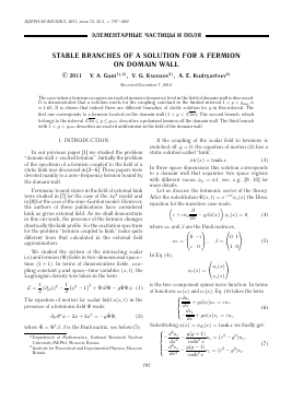
Fig. 1. Slopes a(s) and ß(s).
for s = 2(and g = ^i) with a = a{2) = y2(2 -
The latter case corresponds to the exact solution discussed above, see Eq. (11).
However, Eq. (12) may be used to determine the slope a(s) at x = 0 for the fermionic wave function at arbitrary s G (1; +œ>). The function a(s) is shown in Fig. 1. Note that for large s ^ 1
a(s)
and lim a(s) = 0.
Inserting fermionic wave function (10) with the so obtained a(s) into the r.h.s. of Eq. (2), we get the following equation for the scalar field 0(x):
(Рф
dx2
k3
(13)
a2(s)s^2s - ir(s - 1/2) tanh(a(s)x)
2^T(s - 1)
cosh2s 2(a(s)x)'
This equation has no solutions for boundary conditions (s(0) = 0, d(s(0)/dx = a(s), ( — 1 with x — — at arbitrary s e (1; The only exceptional cases are those with s = 1 and s = 2, for which we found exact solutions discussed above. However, one may try to solve the equation of motion (13) with modified boundary conditions for the field (s(x, 0):
M0) = 0, = (14)
lim (s (x) = 1.
We solved Eq. (13) with boundary conditions (14) numerically, using the shooting method for the whole interval of parameter s e (1; The resultingfunc-tion 3(s) is shown in Fig. 1. Note that 3(s) = = a(s) at two points s = 1 and s = 2, for which our
Ф 1.0
0.8
0.6
0.4
0.2
0 1.0
0.8
0.6
0.4
0.2
0 1.0
0.8
0.6
0.4
0.2
0
5 = 1.5
5 = 5
_i_I_I_I_I_I_I_I_I_I
5 = 10
_i_I_I_I_I_I_I_I_I_I
1 2 3 4 5
x
Fig. 2. Profiles of scalar field 0s (x) at different values of parameter s. Curves: solid — numerical solution of Eq. (13), dashed — approximation of the exact solution by 0S (x) = tanh(^(s)x), dotted — the function (x) = = tanh(a(s)x).
procedure reproduces exact solutions. In the region of small s e (1; 2) functions 3(s) and a(s) do not differ drastically. On the other hand, lim 3(s) = 1, what
s—
means that our solution for scalar field approaches undistorted kink in the limit of large s.
Numerical solutions for the scalar field (s (x) at different values of parameter s are given in Fig. 2, where we also show the profile of the function (s (x) = = tanh(3(s)x). This figure illustrates that for all s e e (1; the exact numerical solution is very close to tanh(3(s)x). So one can say that with high
2
3
4
5
6
1
0
2
6
5
s
ЯДЕРНАЯ ФИЗИКА том 74 №5 2011
e
1.3
E+
a n
10
14
J 18 I_I_I_I_I_I_I_I_I_L
18 ' 2 6 10 14 18
s s
Fig. 3. (a) the energy of the fermion field e(s); (b) total energy of the system "kink + excited bound fermion" E+ (s) (solid curve), the boundary line of the region "domain wall + fermio
Для дальнейшего прочтения статьи необходимо приобрести полный текст. Статьи высылаются в формате PDF на указанную при оплате почту. Время доставки составляет менее 10 минут. Стоимость одной статьи — 150 рублей.